Plot cleaned data overlay overall occurrence data to demonstrate accepted ranges of spatial and non-spatial attributes

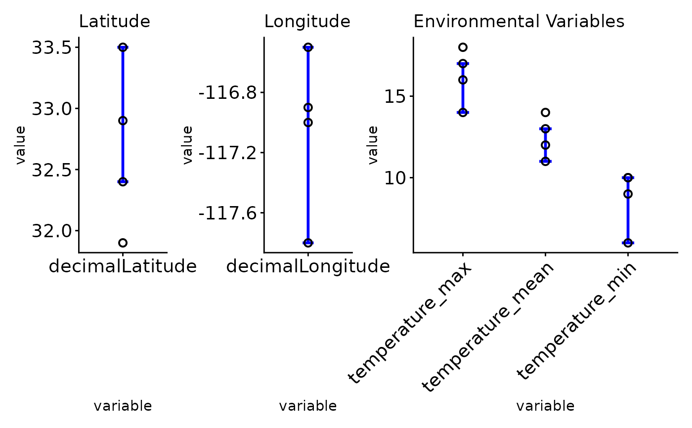
Plot cleaned data overlay overall occurrence data to demonstrate accepted ranges of spatial and non-spatial attributes

Usage

ec_plot_var_range(
  data,
  summary_df,
  latitude = "decimalLatitude",
  longitude = "decimalLongitude",
  env_layers
)

Arguments

data

data table which even has outlier data points

summary_df

summmary output of final cleaned data, after executing function ec_var_summary

latitude

default set to "decimalLatitude"

longitude

default set to "decimalLongitude"

env_layers

list of environmental variables

Value

A plot which shows spatial and environmental variables with the acceptable range for species habitability

Examples

data <- data.frame(
  scientificName = "Mexacanthina lugubris",
  decimalLongitude = c(-117, -117.8, -116.9, -116.5),
  decimalLatitude = c(32.9, 33.5, 31.9, 32.4),
  temperature_mean = c(12, 13, 14, 11),
  temperature_min = c(9, 6, 10, 10),
  temperature_max = c(14, 16, 18, 17),
  flag_outlier = c(0, 0.5, 1, 0.7)
) # this data table has data points which was considered as outliers

data_x <- data.frame(
  scientificName = "Mexacanthina lugubris",
  decimalLongitude = c(-117, -117.8, -116.5),
  decimalLatitude = c(32.9, 33.5, 32.4),
  temperature_mean = c(12, 13, 11),
  temperature_min = c(9, 6, 10),
  temperature_max = c(14, 16, 17),
  flag_outlier = c(0, 0.5, 0.7)
)
# cleaned data base after removing outliers >x probability.
# in this example, removed data points >0.7 probability to be
# considering outliers


env_layers <- c("temperature_mean", "temperature_min", "temperature_max")
summary_df <- ec_var_summary(data_x,
  latitude = "decimalLatitude",
  longitude = "decimalLongitude",
  env_layers
)
# this is the final cleaned data table which
# will be used to derive summary of acceptable niche

ec_plot_var_range(data,
  summary_df,
  latitude = "decimalLatitude",
  longitude = "decimalLongitude",
  env_layers
)